Introduction
This package can be used to process and analyze mass spec data generated by DIANN. It mainly uses the DEP package under the hood, so you can use all DEP functions once you have created the summarizedExperiment object (check out the DEP vignette). Also included are some visualization function that I prefer over the default DEP options.
Installation
Install and load the package from github with the following code (you can ignore the warnings):
if (!require('BiocManager', quietly = T)){
  install.packages('BiocManager')
}

if (!require('devtools', quietly = T)){
  install.packages('devtools')
}

install_github('DijkJel/DIANNmv')
library(DIANNmv)
#> Warning: replacing previous import 'GSEABase::intersect' by
#> 'S4Vectors::intersect' when loading 'DIANNmv'
#> Warning: replacing previous import 'GSEABase::setdiff' by 'S4Vectors::setdiff'
#> when loading 'DIANNmv'
#> Warning: replacing previous import 'S4Vectors::cor' by 'stats::cor' when
#> loading 'DIANNmv'
#> Warning: replacing previous import 'S4Vectors::cov' by 'stats::cov' when
#> loading 'DIANNmv'
#> Warning: replacing previous import 'SummarizedExperiment::start' by
#> 'stats::start' when loading 'DIANNmv'
#> Warning: replacing previous import 'S4Vectors::window' by 'stats::window' when
#> loading 'DIANNmv'
#> Warning: replacing previous import 'S4Vectors::complete.cases' by
#> 'stats::complete.cases' when loading 'DIANNmv'
#> Warning: replacing previous import 'SummarizedExperiment::end' by 'stats::end'
#> when loading 'DIANNmv'
#> Warning: replacing previous import 'MsCoreUtils::smooth' by 'stats::smooth'
#> when loading 'DIANNmv'
#> Warning: replacing previous import 'S4Vectors::var' by 'stats::var' when
#> loading 'DIANNmv'
#> Warning: replacing previous import 'S4Vectors::xtabs' by 'stats::xtabs' when
#> loading 'DIANNmv'
#> Warning: replacing previous import 'S4Vectors::aggregate' by 'stats::aggregate'
#> when loading 'DIANNmv'
#> Warning: replacing previous import 'S4Vectors::na.omit' by 'stats::na.omit'
#> when loading 'DIANNmv'
#> Warning: replacing previous import 'S4Vectors::sd' by 'stats::sd' when loading
#> 'DIANNmv'
#> Warning: replacing previous import 'S4Vectors::na.exclude' by
#> 'stats::na.exclude' when loading 'DIANNmv'
library(SummarizedExperiment)
#> Loading required package: MatrixGenerics
#> Loading required package: matrixStats
#>
#> Attaching package: 'MatrixGenerics'
#> The following objects are masked from 'package:matrixStats':
#>
#>     colAlls, colAnyNAs, colAnys, colAvgsPerRowSet, colCollapse,
#>     colCounts, colCummaxs, colCummins, colCumprods, colCumsums,
#>     colDiffs, colIQRDiffs, colIQRs, colLogSumExps, colMadDiffs,
#>     colMads, colMaxs, colMeans2, colMedians, colMins, colOrderStats,
#>     colProds, colQuantiles, colRanges, colRanks, colSdDiffs, colSds,
#>     colSums2, colTabulates, colVarDiffs, colVars, colWeightedMads,
#>     colWeightedMeans, colWeightedMedians, colWeightedSds,
#>     colWeightedVars, rowAlls, rowAnyNAs, rowAnys, rowAvgsPerColSet,
#>     rowCollapse, rowCounts, rowCummaxs, rowCummins, rowCumprods,
#>     rowCumsums, rowDiffs, rowIQRDiffs, rowIQRs, rowLogSumExps,
#>     rowMadDiffs, rowMads, rowMaxs, rowMeans2, rowMedians, rowMins,
#>     rowOrderStats, rowProds, rowQuantiles, rowRanges, rowRanks,
#>     rowSdDiffs, rowSds, rowSums2, rowTabulates, rowVarDiffs, rowVars,
#>     rowWeightedMads, rowWeightedMeans, rowWeightedMedians,
#>     rowWeightedSds, rowWeightedVars
#> Loading required package: GenomicRanges
#> Loading required package: stats4
#> Loading required package: BiocGenerics
#> Loading required package: generics
#>
#> Attaching package: 'generics'
#> The following objects are masked from 'package:base':
#>
#>     as.difftime, as.factor, as.ordered, intersect, is.element, setdiff,
#>     setequal, union
#>
#> Attaching package: 'BiocGenerics'
#> The following objects are masked from 'package:stats':
#>
#>     IQR, mad, sd, var, xtabs
#> The following objects are masked from 'package:base':
#>
#>     anyDuplicated, aperm, append, as.data.frame, basename, cbind,
#>     colnames, dirname, do.call, duplicated, eval, evalq, Filter, Find,
#>     get, grep, grepl, is.unsorted, lapply, Map, mapply, match, mget,
#>     order, paste, pmax, pmax.int, pmin, pmin.int, Position, rank,
#>     rbind, Reduce, rownames, sapply, saveRDS, table, tapply, unique,
#>     unsplit, which.max, which.min
#> Loading required package: S4Vectors
#>
#> Attaching package: 'S4Vectors'
#> The following object is masked from 'package:utils':
#>
#>     findMatches
#> The following objects are masked from 'package:base':
#>
#>     expand.grid, I, unname
#> Loading required package: IRanges
#> Loading required package: GenomeInfoDb
#> Loading required package: Biobase
#> Welcome to Bioconductor
#>
#>     Vignettes contain introductory material; view with
#>     'browseVignettes()'. To cite Bioconductor, see
#>     'citation("Biobase")', and for packages 'citation("pkgname")'.
#>
#> Attaching package: 'Biobase'
#> The following object is masked from 'package:MatrixGenerics':
#>
#>     rowMedians
#> The following objects are masked from 'package:matrixStats':
#>
#>     anyMissing, rowMedians
library(ggplot2)
Required input data & example data
As input files you will need the protein (report.pg_matrix) and peptide (report.pr_matrix) DIANN output files. In addition, you need an experimental design table. This package comes with these files from a DNA pull down experiment for demonstration goals.You can inspect the data with ‘expDesign’, ‘report.pg_matrix’, and’report.pr_matrix’.
head(report.pg_matrix)
#>                  Protein.Group                      Protein.Names
#> 1 A0A075B6H7;A0A0C4DH55;P01624 KV315_HUMAN;KV37_HUMAN;KVD07_HUMAN
#> 2            A0A0A0MRZ8;P04433            KV311_HUMAN;KVD11_HUMAN
#> 3            A0A0B4J2D5;P0DPI2            GAL3A_HUMAN;GAL3B_HUMAN
#> 4                       A0A183                        LCE6A_HUMAN
#> 5                   A0A1B0GTR4                        SPRR5_HUMAN
#> 6                   A0A1B0GTU1                        ZC11B_HUMAN
#>                       Genes
#> 1 IGKV3-15;IGKV3-7;IGKV3D-7
#> 2        IGKV3-11;IGKV3D-11
#> 3              GATD3;GATD3B
#> 4                     LCE6A
#> 5                     SPRR5
#> 6                   ZC3H11B
#>                                                                      First.Protein.Description
#> 1                                    Probable non-functional immunoglobulin kappa variable 3-7
#> 2                                                          Immunoglobulin kappa variable 3D-11
#> 3 Putative glutamine amidotransferase-like class 1 domain-containing protein 3B, mitochondrial
#> 4                                                           Late cornified envelope protein 6A
#> 5                                                        Putative small proline-rich protein 5
#> 6                                               Zinc finger CCCH domain-containing protein 11B
#>   neg_ctrl_1 neg_ctrl_2 neg_ctrl_3 motif1_1 motif1_2 motif1_3 motif2_1 motif2_2
#> 1    35045.4         NA         NA  60838.8 56361.50  45830.7       NA  41375.0
#> 2    13531.4         NA         NA  26054.8       NA  50914.5  20547.4       NA
#> 3    50098.9   36549.70    43047.0  29253.3 25503.00  47893.5  36321.2  25036.7
#> 4    92060.5   92580.80         NA  49035.6 67543.30  33898.6       NA  33731.9
#> 5    57016.4   58424.50         NA 215301.0 77330.30       NA       NA  69601.4
#> 6    10773.4    9745.44    17668.3  16804.8  9534.48  17388.9  16438.0  25568.2
#>   motif2_3
#> 1 155669.0
#> 2  66331.5
#> 3  28612.7
#> 4       NA
#> 5  47255.0
#> 6       NA
#
#
#
head(report.pr_matrix)
#>   Protein.Group   Protein.Ids Protein.Names  Genes
#> 1        Q86U42        Q86U42   PABP2_HUMAN PABPN1
#> 2        Q8NFD5 Q8NFD5;Q9Y651   ARI1B_HUMAN ARID1B
#> 3        Q96JP5        Q96JP5   ZFP91_HUMAN  ZFP91
#> 4        Q16585        Q16585    SGCB_HUMAN   SGCB
#> 5        P36578        P36578     RL4_HUMAN   RPL4
#> 6        P36578        P36578     RL4_HUMAN   RPL4
#>                          First.Protein.Description Proteotypic
#> 1                  Polyadenylate-binding protein 2           1
#> 2 AT-rich interactive domain-containing protein 1B           0
#> 3                E3 ubiquitin-protein ligase ZFP91           1
#> 4                                 Beta-sarcoglycan           1
#> 5                         60S ribosomal protein L4           1
#> 6                         60S ribosomal protein L4           1
#>     Stripped.Sequence   Modified.Sequence Precursor.Charge         Precursor.Id
#> 1    AAAAAAAAAAGAAGGR    AAAAAAAAAAGAAGGR                2    AAAAAAAAAAGAAGGR2
#> 2         AAAAAAAAAAR         AAAAAAAAAAR                2         AAAAAAAAAAR2
#> 3        AAAAAAAAAVSR        AAAAAAAAAVSR                2        AAAAAAAAAVSR2
#> 4 AAAAAAAAEQQSSNGPVKK AAAAAAAAEQQSSNGPVKK                3 AAAAAAAAEQQSSNGPVKK3
#> 5         AAAAAAALQAK         AAAAAAALQAK                1         AAAAAAALQAK1
#> 6         AAAAAAALQAK         AAAAAAALQAK                2         AAAAAAALQAK2
#>   neg_ctrl_1 neg_ctrl_2 neg_ctrl_3    motif1_1   motif1_2   motif1_3
#> 1    14201.4    17402.1    22342.6     9617.31    12355.2    10824.8
#> 2 56500900.0 59560000.0 64613700.0 51690200.00 23066300.0 40866800.0
#> 3 12186100.0 12535000.0 15420900.0 28513800.00 32014600.0 43538700.0
#> 4         NA         NA         NA     8669.59         NA         NA
#> 5  3729720.0  4311790.0  2780390.0  3405560.00  4964600.0  4373450.0
#> 6 71649900.0 31629500.0 43972100.0 67226000.00 48326400.0 47199700.0
#>      motif2_1 motif2_2    motif2_3
#> 1    11469.50    11064     9728.03
#> 2 30508900.00 30926500 39211400.00
#> 3 41882400.00 53996100 30695300.00
#> 4     8965.43       NA          NA
#> 5  6242340.00  3104850  6942140.00
#> 6 32204200.00 40380400 39495700.00
#
#
#
expDesign
#>        label condition replicate
#> 1 neg_ctrl_1  neg_ctrl         1
#> 2 neg_ctrl_2  neg_ctrl         2
#> 3 neg_ctrl_3  neg_ctrl         3
#> 4   motif1_1    motif1         1
#> 5   motif1_2    motif1         2
#> 6   motif1_3    motif1         3
#> 7   motif2_1    motif2         1
#> 8   motif2_2    motif2         2
#> 9   motif2_3    motif2         3
As you can see in expDesign, there are three conditions with 3 replicates each: Two variations of a TF binding motif and one negative control that can be used for both motifs. The names in the ‘label’ column correspond to the intensity columns in report.pg_matrix and should be in the same order and identically named.
Prepare input data
If the sample names in the report.pg_matrix and report.pr_matrix are
structured like
tidy_data <- prepare_diann_data(report.pg_matrix, report.pr_matrix)
#> Warning in max(which(!selection == T)): no non-missing arguments to max;
#> returning -Inf
#> Warning in colnames(pr_matrix)[start_index_pr:ncol(pr_matrix)] <- cn: number of
#> items to replace is not a multiple of replacement length
#>                 label condition replicate
#> neg_ctrl_3 neg_ctrl_3  neg_ctrl         3
#> motif1_1     motif1_1    motif1         1
#> motif1_2     motif1_2    motif1         2
#> motif1_3     motif1_3    motif1         3
#> motif2_1     motif2_1    motif2         1
#> motif2_2     motif2_2    motif2         2
#> motif2_3     motif2_3    motif2         3
pg_matrix <- tidy_data$pg_matrix
pr_matrix <- tidy_data$pr_matrix
Prepare the Summarized Experiment object
The report.pg_matrix, report.pr_matrix and expDesign are combined in a summarizedExperiment (se) object that is used for downstream analysis and plotting.
To create an se object, you can run the prepare_se() function with the report.pg_matrix file and associated experimental design. You can specify if and what type of imputation is done. The default is ‘mixed’, which uses both missing-not-at-random (MNAR) and missing-at-random (MAR) imputation. For MNAR/MAR specific imputation, ‘knn’ and ‘MinProb’ are advised, respectively. When ‘none’ is entered for the impute parameter, no imputation is done. Additionally, you can filter on missing values (missing_thr), and potential contaminants are removed by default. (Source: contaminants.txt file from maxquant).
se <- prepare_se(report.pg_matrix, expDesign) # without peptide information
#> Imputing along margin 2 (samples/columns).
#> [1] 0.3066195
#> Imputing along margin 1 (features/rows).
#> Warning in knnimp(x, k, maxmiss = rowmax, maxp = maxp): 36 rows with more than 50 % entries missing;
#>  mean imputation used for these rows
#> Cluster size 5574 broken into 2304 3270
#> Cluster size 2304 broken into 720 1584
#> Done cluster 720
#> Cluster size 1584 broken into 953 631
#> Done cluster 953
#> Done cluster 631
#> Done cluster 1584
#> Done cluster 2304
#> Cluster size 3270 broken into 1239 2031
#> Done cluster 1239
#> Cluster size 2031 broken into 1024 1007
#> Done cluster 1024
#> Done cluster 1007
#> Done cluster 2031
#> Done cluster 3270
se
#> class: SummarizedExperiment
#> dim: 5610 9
#> metadata(0):
#> assays(2): '' imputation_mask
#> rownames(5610): A2M A2ML1 ... ZYX ZZZ3
#> rowData names(7): Protein.Group Protein.Names ... name ID
#> colnames(9): neg_ctrl_1 neg_ctrl_2 ... motif2_2 motif2_3
#> colData names(4): label ID condition replicate
If you provide the report.pr_matrix alongside the report.pg_matrix, peptide information is automatically added and you can filter on a minimal number of razor/unique peptides (min_pep, default = 1). Make sure the sample column names are identical and match the label column in the experimental design.
# Add peptide information and remove all proteinGroups with <2 total
# razor/unique peptides
se <- prepare_se(report.pg_matrix, expDesign, report.pr_matrix, min_pep = 2)
#> Imputing along margin 2 (samples/columns).
#> [1] 0.2979843
#> Imputing along margin 1 (features/rows).
#> Warning in knnimp(x, k, maxmiss = rowmax, maxp = maxp): 19 rows with more than 50 % entries missing;
#>  mean imputation used for these rows
#> Cluster size 5260 broken into 3646 1614
#> Cluster size 3646 broken into 2279 1367
#> Cluster size 2279 broken into 1220 1059
#> Done cluster 1220
#> Done cluster 1059
#> Done cluster 2279
#> Done cluster 1367
#> Done cluster 3646
#> Cluster size 1614 broken into 1176 438
#> Done cluster 1176
#> Done cluster 438
#> Done cluster 1614
se
#> class: SummarizedExperiment
#> dim: 5279 9
#> metadata(1): pr_matrix
#> assays(3): '' peptide_info imputation_mask
#> rownames(5279): A2M A2ML1 ... ZYX ZZZ3
#> rowData names(9): Protein.Group Protein.Names ... ID npep_total
#> colnames(9): neg_ctrl_1 neg_ctrl_2 ... motif2_2 motif2_3
#> colData names(4): label ID condition replicate
The summarizedExperiment object stores a lot of information. As you can see from the output above, it consists of 5584 proteinGroups (rows) and 9 samples (columns). Furthermore, the experimental design is stored as ‘colData’, and extra information is stored as ‘rowData’. The log2 transformed intensities form the main assay. Furthermore, if the report.pr_matrix file was provided, a second assay is added. For a detailed description of the structure of summarizedExperiments, check its documentation. In short, to access different parts of data:
intensities <- assay(se) # log2 protein intensities
peptides <- assay(se, 'peptide_info') # peptide numbers

rd = as.data.frame(rowData(se))
colnames(rd) # Information for each proteinGroup in the se.
#> [1] "Protein.Group"             "Protein.Names"
#> [3] "Genes"                     "First.Protein.Description"
#> [5] "n_total"                   "Potential.contaminant"
#> [7] "name"                      "ID"
#> [9] "npep_total"

cd = as.data.frame(colData(se))
cd # The experimental design
#>                 label         ID condition replicate
#> neg_ctrl_1 neg_ctrl_1 neg_ctrl_1  neg_ctrl         1
#> neg_ctrl_2 neg_ctrl_2 neg_ctrl_2  neg_ctrl         2
#> neg_ctrl_3 neg_ctrl_3 neg_ctrl_3  neg_ctrl         3
#> motif1_1     motif1_1   motif1_1    motif1         1
#> motif1_2     motif1_2   motif1_2    motif1         2
#> motif1_3     motif1_3   motif1_3    motif1         3
#> motif2_1     motif2_1   motif2_1    motif2         1
#> motif2_2     motif2_2   motif2_2    motif2         2
#> motif2_3     motif2_3   motif2_3    motif2         3
Note on integration with the DEP package
If your experimental design and sample labels follow the convention
of
se_dep <- use_dep(se)Add peptide and iBAQ information
The report.pr_matrix and report.pg_matrix files can be used to add peptide number information, iBAQ values, and median peptide intensities, which are an alternative to iBAQ.
Add number of razor/unique peptides
This information is automatically added to the se object when running prepare_se() and providing a report.pr_matrix file (see above). You can also manually add this to the report.pg_matrix() file with the following code.
To get the number of razor/unique peptides per proteinGroup per sample and the total number of razor/unique peptides over all samples, and add these to the report.pg_matrix file:
peptides <- get_nPep_prMatrix(report.pr_matrix)
pg_matrix <- add_peptide_numbers(report.pg_matrix, peptides)
This adds new columns with the suffix ‘npep’ to the report.pg_matrix with the number of identified peptides per sample, and ‘n_total’ with the total number of identified razor/unique peptides per proteinGroup.
colnames(pg_matrix)
#>  [1] "Protein.Group"             "Protein.Names"
#>  [3] "Genes"                     "First.Protein.Description"
#>  [5] "neg_ctrl_1"                "neg_ctrl_2"
#>  [7] "neg_ctrl_3"                "motif1_1"
#>  [9] "motif1_2"                  "motif1_3"
#> [11] "motif2_1"                  "motif2_2"
#> [13] "motif2_3"                  "neg_ctrl_1_npep"
#> [15] "neg_ctrl_2_npep"           "neg_ctrl_3_npep"
#> [17] "motif1_1_npep"             "motif1_2_npep"
#> [19] "motif1_3_npep"             "motif2_1_npep"
#> [21] "motif2_2_npep"             "motif2_3_npep"
#> [23] "n_total"
Add iBAQ data
iBAQ values can be added to the pg_matrix file as well. For that, we need the number of theoretically observable peptides, and non-normalized intensities.
The number of iBAQ peptides for reviewed human and mouse uniprot entries are included in the package and can be accessed with:
ibaq_peptides <- DIANNmv::ibaq_peptides
hs <- ibaq_peptides$hs #Human entries
mm <- ibaq_peptides$mm # Mouse entries
If you do not want to use these, you can create an similar object yourself from a fasta file:
no_ibaq_peptides <- get_ibaq_peptides('path/to/fasta.fasta')Non-normalized intensities can be calculated as sum of individual peptide intensites from the report.pr_matrix file:
intensities <- get_intensities_prMatrix(report.pr_matrix)This is all combined in the the add_iBAQ() function, which addes columns with iBAQ values and a column with the number of iBAQ peptides to the report.pg_matrix. If you use the included iBAQ peptides, you only have to specify the organism. If you use a custom file, you have to specify it with the ‘ibaq_stats’ parameter.
pg <- add_iBAQ(report.pg_matrix, report.pr_matrix, organism = 'hs') # Standard
colnames(pg)
#>  [1] "Protein.Group"             "Protein.Names"
#>  [3] "Genes"                     "First.Protein.Description"
#>  [5] "neg_ctrl_1"                "neg_ctrl_2"
#>  [7] "neg_ctrl_3"                "motif1_1"
#>  [9] "motif1_2"                  "motif1_3"
#> [11] "motif2_1"                  "motif2_2"
#> [13] "motif2_3"                  "neg_ctrl_1_iBAQ"
#> [15] "neg_ctrl_2_iBAQ"           "neg_ctrl_3_iBAQ"
#> [17] "motif1_1_iBAQ"             "motif1_2_iBAQ"
#> [19] "motif1_3_iBAQ"             "motif2_1_iBAQ"
#> [21] "motif2_2_iBAQ"             "motif2_3_iBAQ"
#> [23] "ibaq_peptides"
The iBAQ values are automatically added to the
summarizedExperiment object when running the prepare_se() function. In
addition, the number of iBAQ peptides is added to the rowData.
pg <- add_iBAQ(report.pg_matrix, report.pr_matrix, organism = 'hs')
se <- prepare_se(pg, expDesign, report.pr_matrix)
#> Imputing along margin 2 (samples/columns).
#> [1] 0.3059733
#> Imputing along margin 1 (features/rows).
#> Warning in knnimp(x, k, maxmiss = rowmax, maxp = maxp): 33 rows with more than 50 % entries missing;
#>  mean imputation used for these rows
#> Cluster size 5500 broken into 3626 1874
#> Cluster size 3626 broken into 1266 2360
#> Done cluster 1266
#> Cluster size 2360 broken into 1196 1164
#> Done cluster 1196
#> Done cluster 1164
#> Done cluster 2360
#> Done cluster 3626
#> Cluster size 1874 broken into 1281 593
#> Done cluster 1281
#> Done cluster 593
#> Done cluster 1874
iBAQ <- as.matrix(assay(se, 'iBAQ'))
head(iBAQ)
#>       neg_ctrl_1  neg_ctrl_2 neg_ctrl_3   motif1_1  motif1_2  motif1_3
#> A2M    44908.143  43355.8406   64753.94  41528.739 123416.60  21931.53
#> A2ML1 112836.227 154355.9719   88353.84 136172.283 135247.20 156184.82
#> AAAS  595275.548 778864.7519  733462.15 248484.556 725698.24 489673.48
#> AAK1   24854.583    126.1392   26950.56  23150.526  19485.50  22769.03
#> AAR2   29334.317 183248.0889   39214.12   3291.122  35568.44  33472.99
#> AARS1   3359.781  10436.0490       0.00      0.000   2132.97   2367.20
#>         motif2_1  motif2_2   motif2_3
#> A2M     4432.100 108122.55  85534.064
#> A2ML1  47171.734  77564.26 106892.719
#> AAAS  278873.133 263530.63 505940.196
#> AAK1       0.000      0.00  21978.459
#> AAR2  201094.172 108991.24 177086.150
#> AARS1   1908.576   3763.05   2011.761

ibaq_pep <- rowData(se)$ibaq_peptides
head(ibaq_pep)
#> [1] 69 64 27 36 18 50
Add median peptide intensities
Similarly, median peptide intensities (mpi) can be added. To get the mpi as separate object:
mpi <- get_median_intensities_prMatrix(report.pr_matrix)
head(mpi)
#>                        protein neg_ctrl_1 neg_ctrl_2 neg_ctrl_3  motif1_1
#> 1 A0A075B6H7;A0A0C4DH55;P01624    35045.4         NA         NA  60838.90
#> 2            A0A0A0MRZ8;P04433    13531.4    5577.47         NA  26054.80
#> 3            A0A0B4J2D5;P0DPI2    31083.5   23493.25    17767.3  18834.27
#> 4                       A0A183    74635.8   96073.55         NA  64140.95
#> 5                   A0A1B0GTR4    56976.9   58384.00         NA 148435.10
#> 6                   A0A1B0GTU1   255493.0    9745.44    17668.3  16804.80
#>    motif1_2 motif1_3 motif2_1 motif2_2  motif2_3
#> 1  56361.40  45830.7       NA  41375.0 155669.00
#> 2  25558.50  50914.5  20547.4       NA  66331.50
#> 3 249944.00  21172.3  25210.3 192574.0 267984.40
#> 4  78935.65  82479.8       NA  78484.7        NA
#> 5  47525.95       NA  65137.5  71409.6  23997.25
#> 6   9534.49  17388.9  16438.0  25568.2   8499.39
To add mpi to the se object directly (this requires that the se includes the pr_matrix when running prepare_se()):
 se <- add_median_peptide_intensity(se)
 se # an extra assay 'median_peptide_intensities' is added
#> class: SummarizedExperiment
#> dim: 5533 9
#> metadata(1): pr_matrix
#> assays(6): '' iBAQ ... imputation_mask median_peptide_intensities
#> rownames(5533): A2M A2ML1 ... ZYX ZZZ3
#> rowData names(11): Protein.Group Protein.Names ... npep_total
#>   baseMean_mpi
#> colnames(9): neg_ctrl_1 neg_ctrl_2 ... motif2_2 motif2_3
#> colData names(4): label ID condition replicate
 mpi <- assay(se, 'median_peptide_intensities')

 rd <- as.data.frame(rowData(se))
 head(rd$baseMean_mpi) # shows the average mpi per proteinGroup over all samples
#> [1] 339967.8 366450.2 411634.6 600430.1 307316.9 108054.2
Differential protein analysis
To perform differential protein expression analysis, you have to run the get_DEPresults() function. There are three main types: ‘manual’ (1 vs 1), ‘control’ (all vs 1), and ‘all’ (all vs all). For ‘manual’, you can also specify the contrasts you want to test by providing a character vector for the ‘tests’ parameter.In addition, you can choose the p.adj cutoff and log2 fold change cutoffs for significant, and the method of FDR correction. The DEP default is ‘fdrtool’, but this has given some weird results in the past. Therefore, the default here is ‘BH’ (Benjamini-Hochberg), which is also the default that limma uses (which DEP uses in the background).
get_DEPresults returns a data frame with statistics for the specified tests, and can be used for visualization afterwards.
# To test a 1 vs 1 comparison
res_man <- get_DEPresults(se, condition1 = 'motif1', condition2 = 'neg_ctrl',
                      type = 'manual')
#> Tested contrasts: motif1_vs_neg_ctrl

# To test multiple 1 vs 1 comparisons
res_man2 <- get_DEPresults(se,
                           tests = c('motif1_vs_neg_ctrl', 'motif1_vs_motif2'),
                           type = 'manual')
#> Tested contrasts: motif1_vs_neg_ctrl, motif1_vs_motif2

# To test all conditions vs 1 reference condition
res_ref <- get_DEPresults(se, ref_condition = 'neg_ctrl', type = 'control')
#> Tested contrasts: motif1_vs_neg_ctrl, motif2_vs_neg_ctrl

# To test all vs all
res <- get_DEPresults(se, type = 'all')
#> Tested contrasts: neg_ctrl_vs_motif1, neg_ctrl_vs_motif2, motif1_vs_motif2
Plotting
Protein Coverage
To plot the coverage and intensity of identified peptides of a protein, you can use plot_protein_coverage(). This expects the report.pr_matrix file. You can plot multiple proteins faceted, and highlight amino acid positions in the protein. By default, overlapping peptides (e.g. due to miscleavages) are combined and the intensities are summed.
# The default option
smad4 <- plot_protein_coverage(se, 'SMAD4')
#> Warning: Duplicated aesthetics after name standardisation: ymin
smad4
#> Warning: Duplicated aesthetics after name standardisation: ymin
#> Duplicated aesthetics after name standardisation: ymin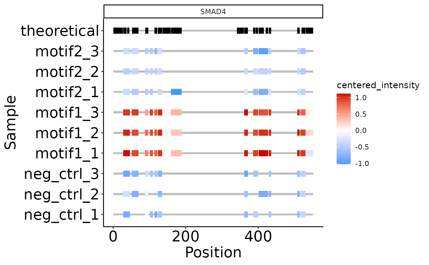
# Indicate amino acid positions and zoom in on aa 50-200 of protein:
smad4_zoom <- plot_protein_coverage(se, 'SMAD4', c(100, 120),
                                    zoom = c(50, 200))
#> Warning: Duplicated aesthetics after name standardisation: ymin
#> Coordinate system already present.
#> ℹ Adding new coordinate system, which will replace the existing one.

smad4_zoom
#> Warning: Duplicated aesthetics after name standardisation: ymin
#> Duplicated aesthetics after name standardisation: ymin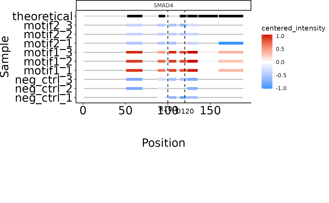
Volcano plots
The plotVolcano() function returns volcano plots with the specified
significance cutoffs. If more than 1 comparison is present in your
results data frame, a list of volcano plots will be returned which can
be accessed by the ‘$’ operator. By default, proteins that have any
imputed values in the two conditions compared will be specified. Check
the help page for plotVolcano() (?plotVolcano) to see the
different options for labeling specific points in the volcano.
plotVolcano(res_man) # Default volcano plot if one comparison is present.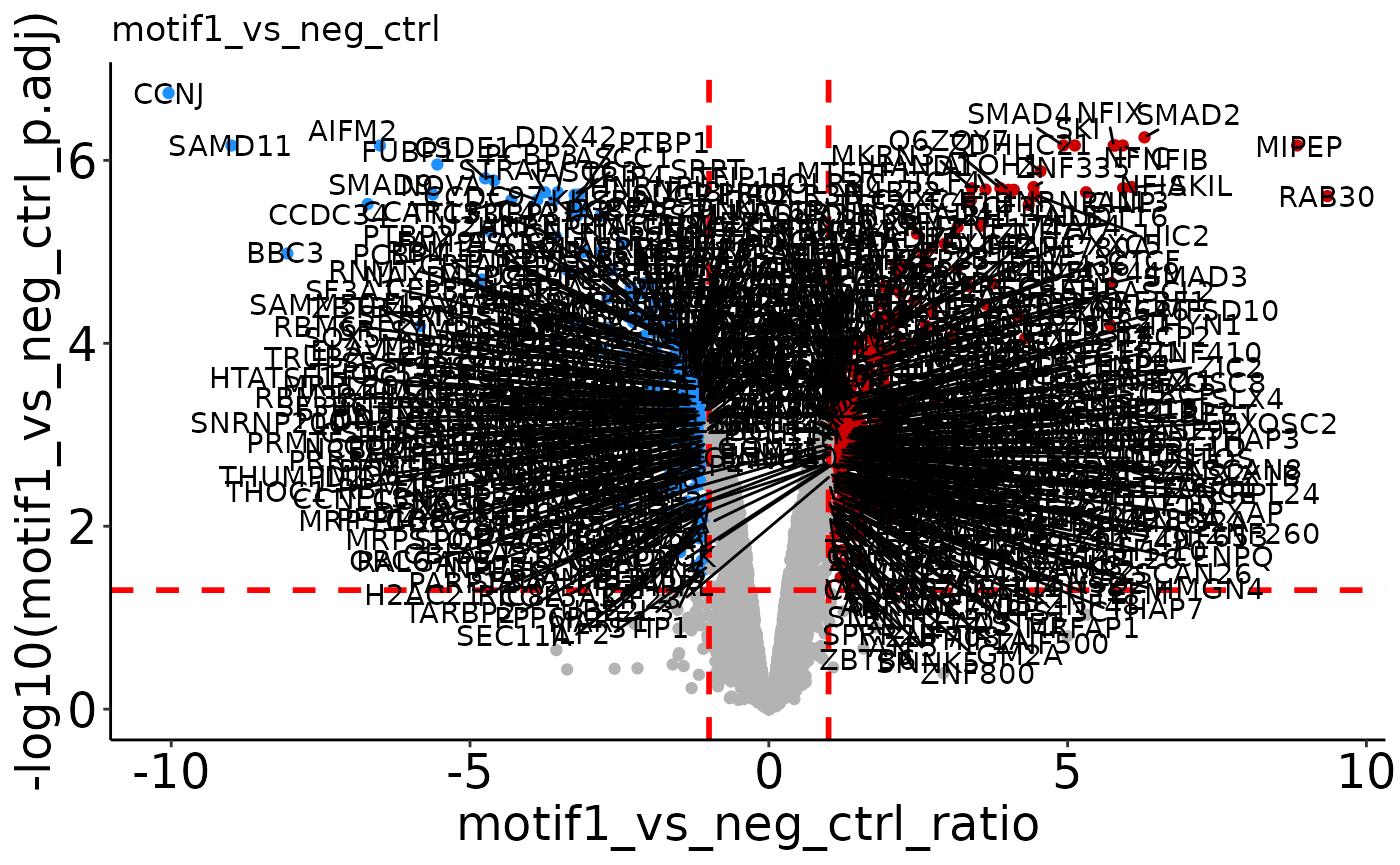
                    # labels all significant points (can be a bit much).


volcano_list <- plotVolcano(res_ref, label = '') # returns list of volcano plots
                                                 # Don't label anything.
volcano_list$motif1_vs_neg_ctrl # Select which plot you want to see.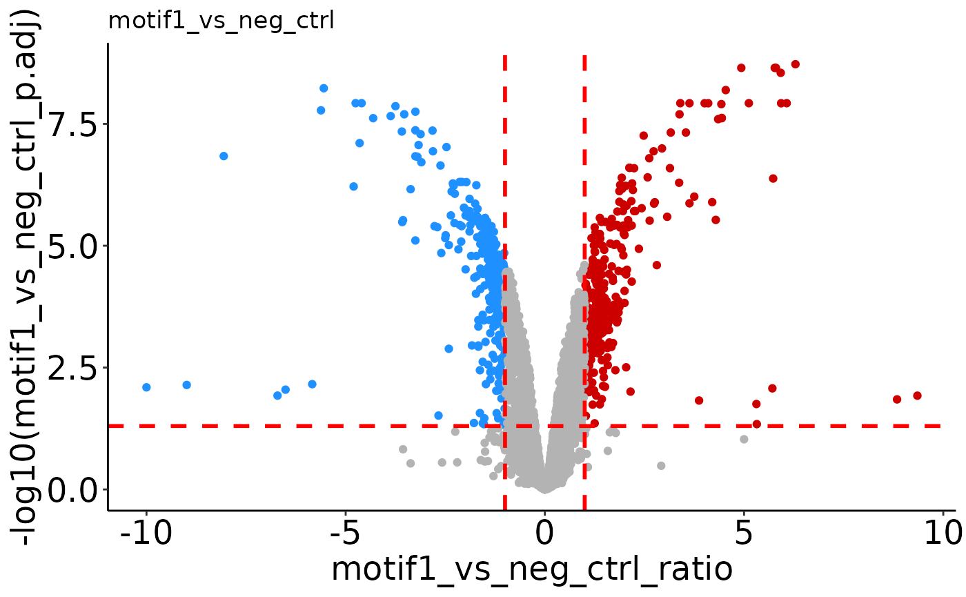
# Example of a very ugly volcano plot.
plotVolcano(res_man, pval_cutoff = 0.001, fc_cutoff = 2,
            up_color =  'blue', down_color = 'yellow', ns_color = 'green',
            label = c('SMAD3', 'SMAD4'))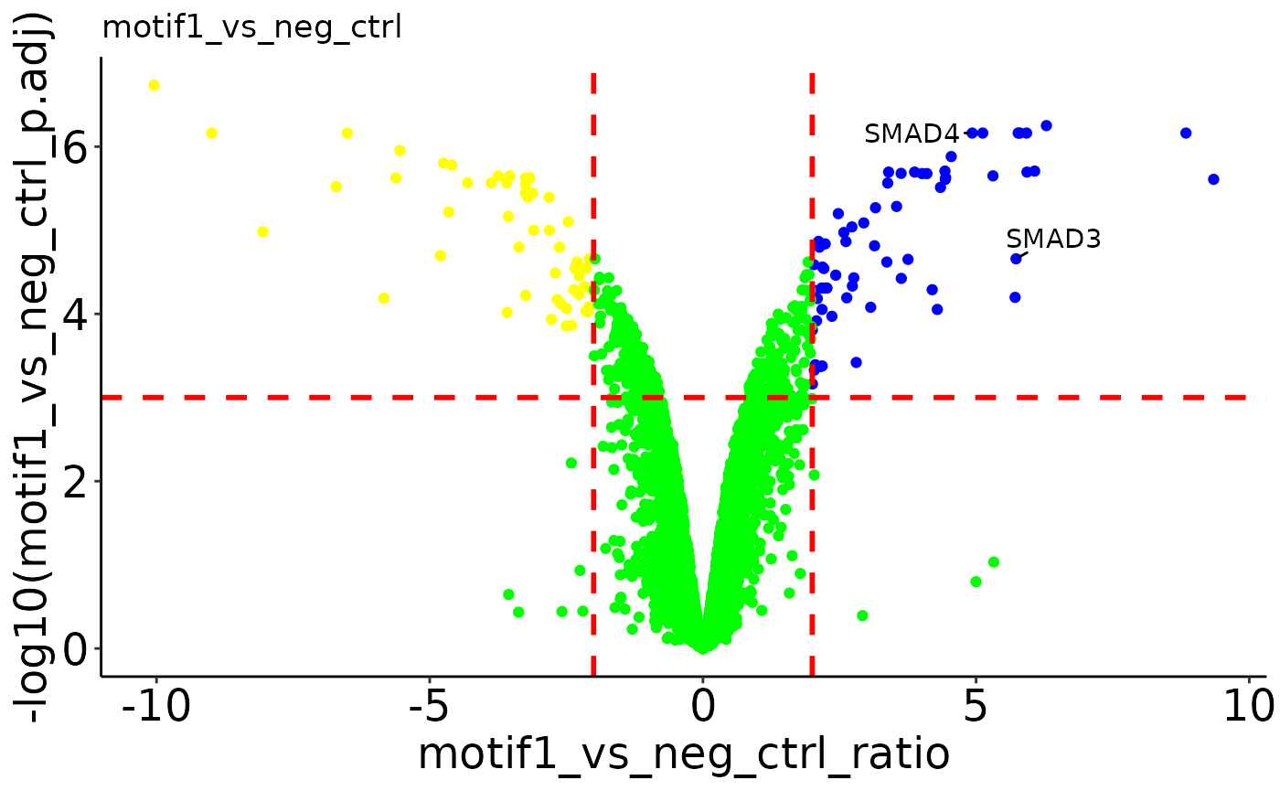
MA-plots
If median_peptide_intensities are added to the se, you can also plot an MA-plot, with abundances on the x-axis, and fold-changes on the y-axis. Significant hits are indicated in blue/red:
plot_MA(res_man, label = c('SMAD3', 'SMAD4'))
#> Warning: Removed 26 rows containing missing values or values outside the scale range
#> (`geom_point()`).
#> Warning: Removed 26 rows containing missing values or values outside the scale range
#> (`geom_text_repel()`).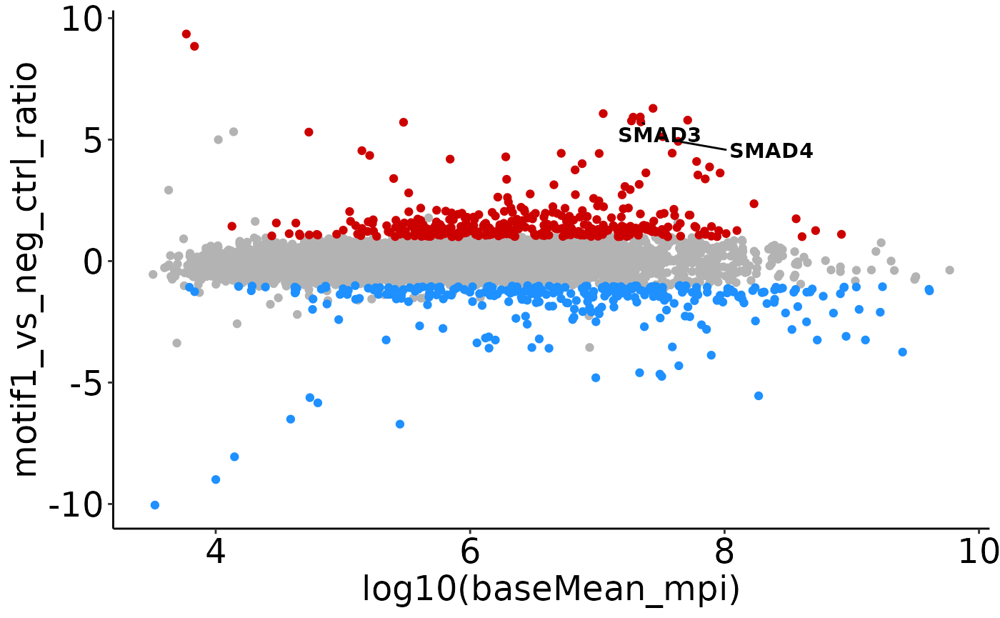
Venn diagrams
You can also make a Venn diagram showing overlapping significant proteins. By default, all comparisons present in your results data frame are used, but it can handle five comparisons maximally. You can specify which comparisons to include.
plot_venn_diagram(res) # all comparisons
#> INFO [2025-10-14 08:01:36] [[1]]
#> INFO [2025-10-14 08:01:36] venn_list
#> INFO [2025-10-14 08:01:36]
#> INFO [2025-10-14 08:01:36] $filename
#> INFO [2025-10-14 08:01:36] NULL
#> INFO [2025-10-14 08:01:36]
#> INFO [2025-10-14 08:01:36] $disable.logging
#> INFO [2025-10-14 08:01:36] T
#> INFO [2025-10-14 08:01:36]
#> INFO [2025-10-14 08:01:36] $fill
#> INFO [2025-10-14 08:01:36] colors
#> INFO [2025-10-14 08:01:36]
#> INFO [2025-10-14 08:01:36] $fontfamily
#> INFO [2025-10-14 08:01:36] [1] "sans"
#> INFO [2025-10-14 08:01:36]
#> INFO [2025-10-14 08:01:36] $fontface
#> INFO [2025-10-14 08:01:36] [1] "bold"
#> INFO [2025-10-14 08:01:36]
#> INFO [2025-10-14 08:01:36] $cat.fontfamily
#> INFO [2025-10-14 08:01:36] [1] "sans"
#> INFO [2025-10-14 08:01:36]
#> INFO [2025-10-14 08:01:36] $lty
#> INFO [2025-10-14 08:01:36] [1] 0
#> INFO [2025-10-14 08:01:36]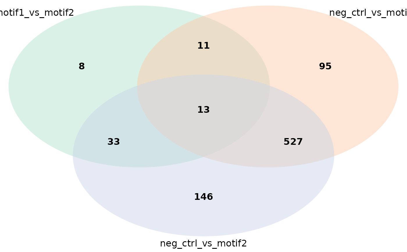
plot_venn_diagram(res, comparisons = c('neg_ctrl_vs_motif1',
                                       'neg_ctrl_vs_motif2')) # only two comp.
#> INFO [2025-10-14 08:01:36] [[1]]
#> INFO [2025-10-14 08:01:36] venn_list
#> INFO [2025-10-14 08:01:36]
#> INFO [2025-10-14 08:01:36] $filename
#> INFO [2025-10-14 08:01:36] NULL
#> INFO [2025-10-14 08:01:36]
#> INFO [2025-10-14 08:01:36] $disable.logging
#> INFO [2025-10-14 08:01:36] T
#> INFO [2025-10-14 08:01:36]
#> INFO [2025-10-14 08:01:36] $fill
#> INFO [2025-10-14 08:01:36] colors
#> INFO [2025-10-14 08:01:36]
#> INFO [2025-10-14 08:01:36] $fontfamily
#> INFO [2025-10-14 08:01:36] [1] "sans"
#> INFO [2025-10-14 08:01:36]
#> INFO [2025-10-14 08:01:36] $fontface
#> INFO [2025-10-14 08:01:36] [1] "bold"
#> INFO [2025-10-14 08:01:36]
#> INFO [2025-10-14 08:01:36] $cat.fontfamily
#> INFO [2025-10-14 08:01:36] [1] "sans"
#> INFO [2025-10-14 08:01:36]
#> INFO [2025-10-14 08:01:36] $lty
#> INFO [2025-10-14 08:01:36] [1] 0
#> INFO [2025-10-14 08:01:36]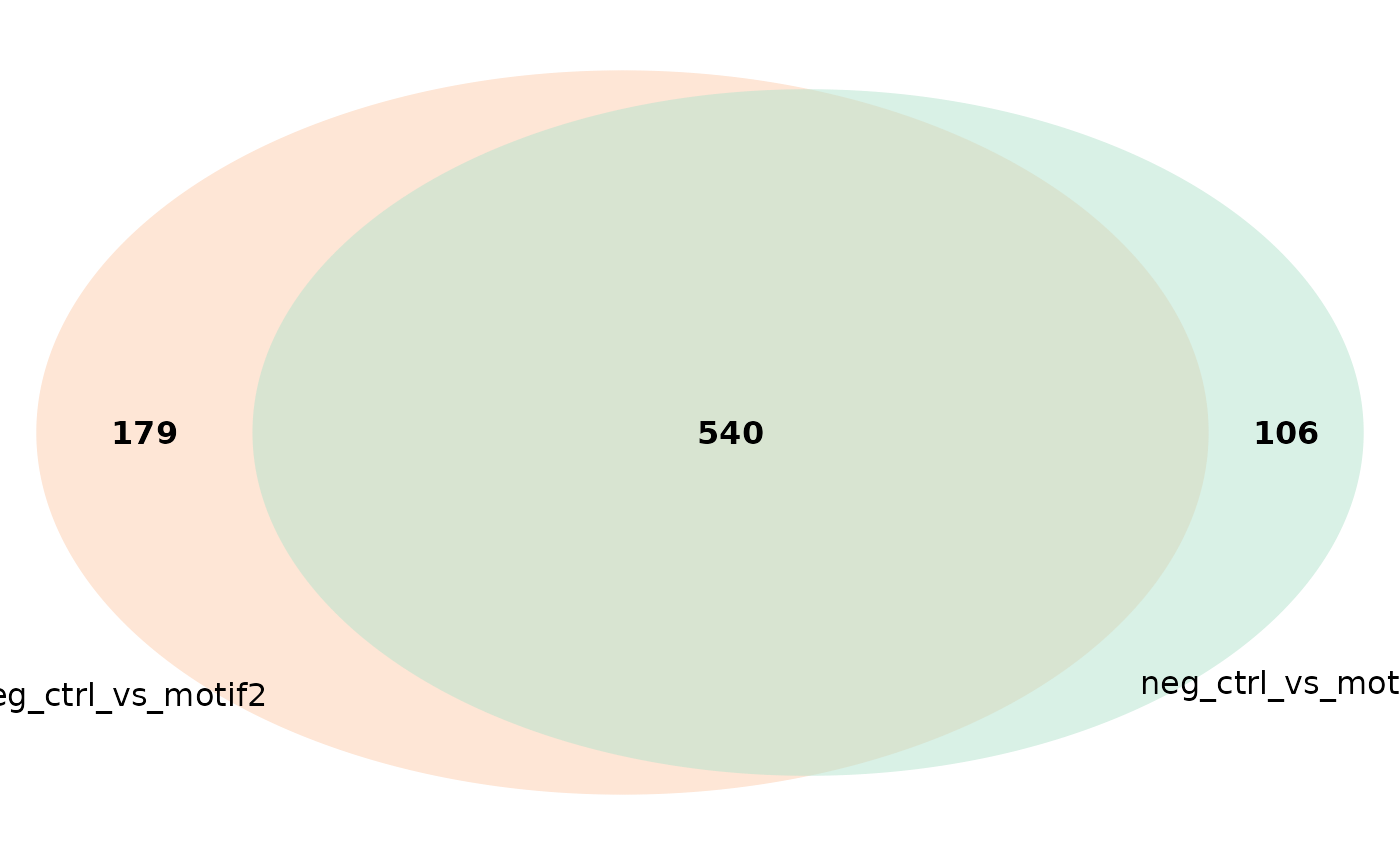
plot_venn_diagram(res, comparisons = c('neg_ctrl_vs_motif1',
                                       'neg_ctrl_vs_motif2'),
                  colors = c('red', 'blue')) # specify colors used
#> INFO [2025-10-14 08:01:36] [[1]]
#> INFO [2025-10-14 08:01:36] venn_list
#> INFO [2025-10-14 08:01:36]
#> INFO [2025-10-14 08:01:36] $filename
#> INFO [2025-10-14 08:01:36] NULL
#> INFO [2025-10-14 08:01:36]
#> INFO [2025-10-14 08:01:36] $disable.logging
#> INFO [2025-10-14 08:01:36] T
#> INFO [2025-10-14 08:01:36]
#> INFO [2025-10-14 08:01:36] $fill
#> INFO [2025-10-14 08:01:36] colors
#> INFO [2025-10-14 08:01:36]
#> INFO [2025-10-14 08:01:36] $fontfamily
#> INFO [2025-10-14 08:01:36] [1] "sans"
#> INFO [2025-10-14 08:01:36]
#> INFO [2025-10-14 08:01:36] $fontface
#> INFO [2025-10-14 08:01:36] [1] "bold"
#> INFO [2025-10-14 08:01:36]
#> INFO [2025-10-14 08:01:36] $cat.fontfamily
#> INFO [2025-10-14 08:01:36] [1] "sans"
#> INFO [2025-10-14 08:01:36]
#> INFO [2025-10-14 08:01:36] $lty
#> INFO [2025-10-14 08:01:36] [1] 0
#> INFO [2025-10-14 08:01:36]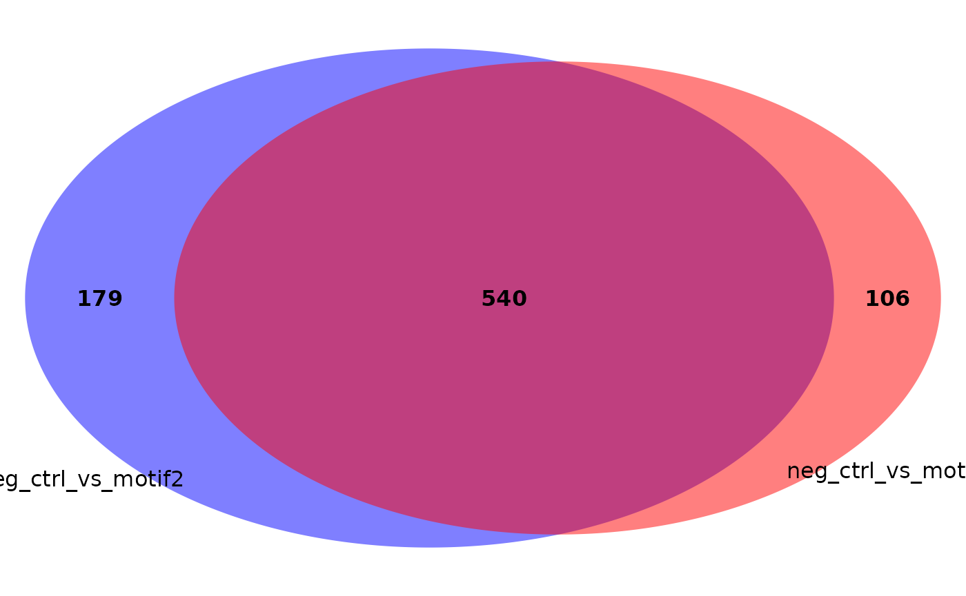
Upset plot
As an alternative to Venn diagrams, you can also plot protein membership as an upset plot. Individual components of the plot can be altered after the plot is made. Check the ‘ggupset’ vignette for instructions on how to do this.
upset_plot <- plot_upset(res)
upset_plot
#> Warning: Using `size` aesthetic for lines was deprecated in ggplot2 3.4.0.
#> ℹ Please use `linewidth` instead.
#> ℹ The deprecated feature was likely used in the ggupset package.
#>   Please report the issue at <https://github.com/const-ae/ggupset/issues>.
#> This warning is displayed once every 8 hours.
#> Call `lifecycle::last_lifecycle_warnings()` to see where this warning was
#> generated.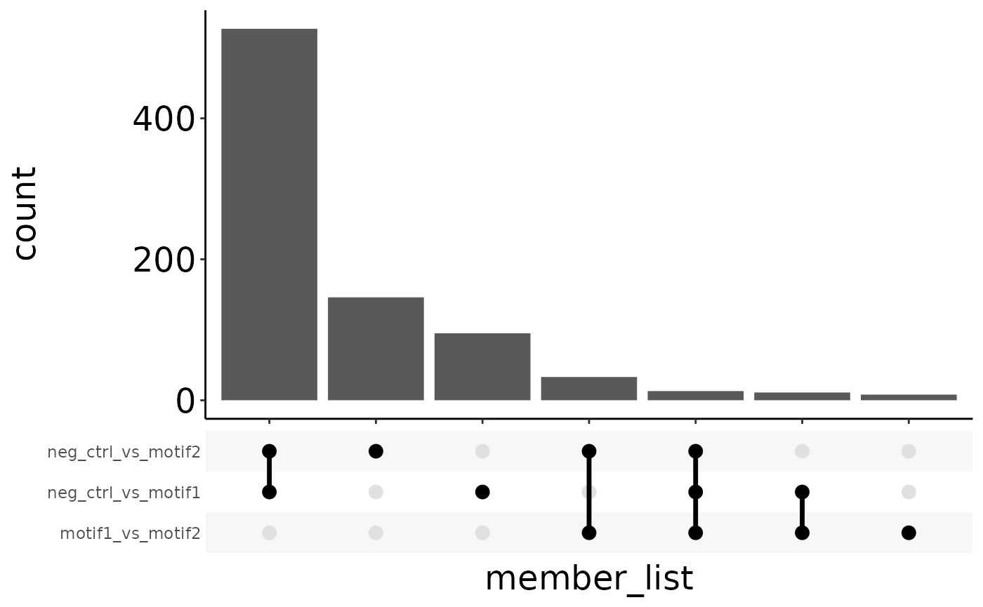
Finally, to get an overview of the number of identified significant proteins per condition:
plot_DEP_barplot(res)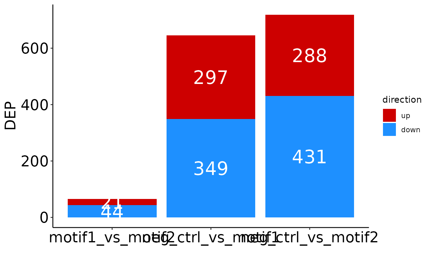
You can change the conditions included, order of columns, and labels:
# Include only two comparisons and change the order:
plot_DEP_barplot(res, comparisons = c('neg_ctrl_vs_motif2',
                                      'neg_ctrl_vs_motif1'))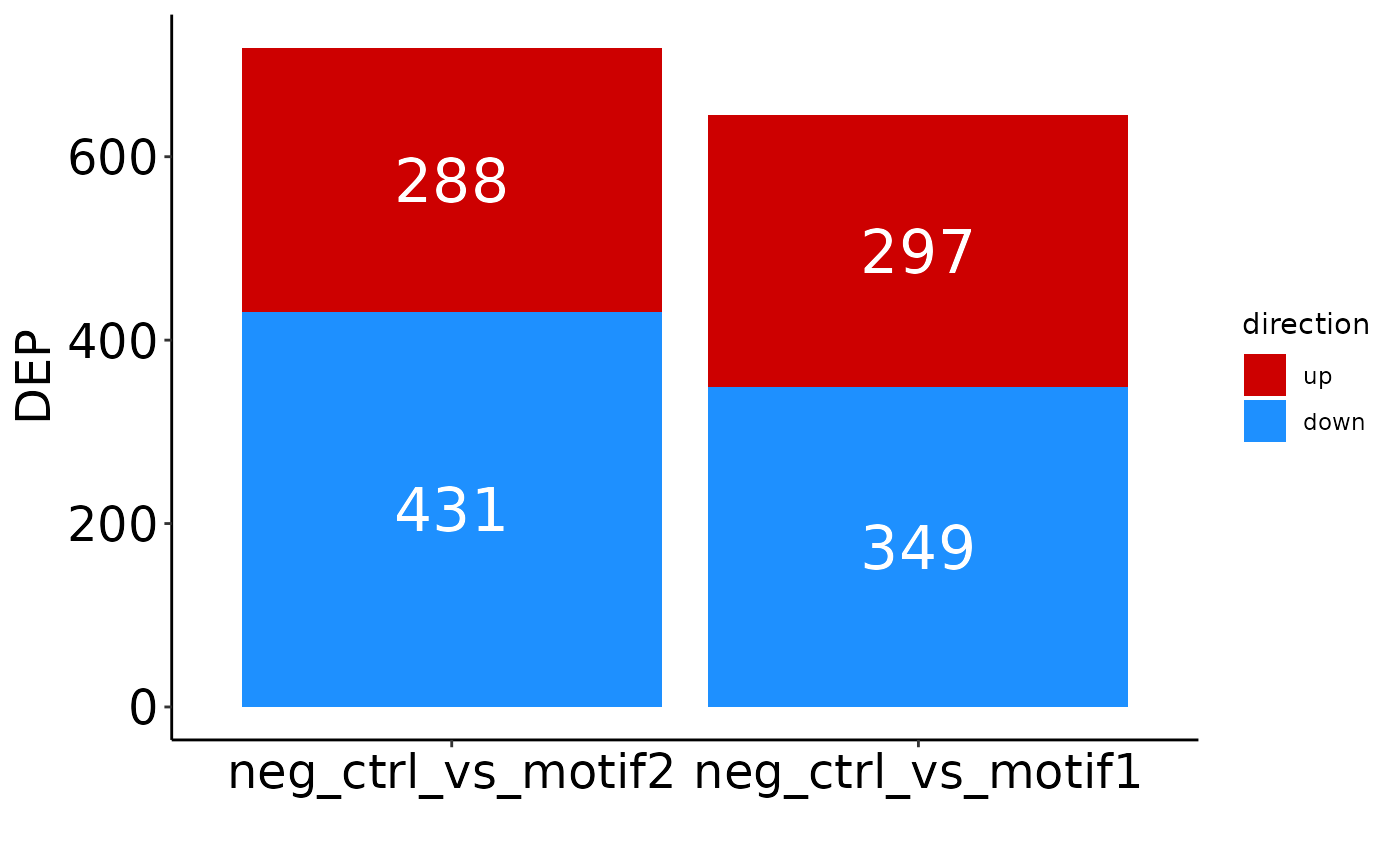
# Same as above, but axis labels are changed.
plot_DEP_barplot(res, comparisons = c('neg_ctrl_vs_motif2',
                                      'neg_ctrl_vs_motif1'),
                 names = c('motif2', 'motif1'))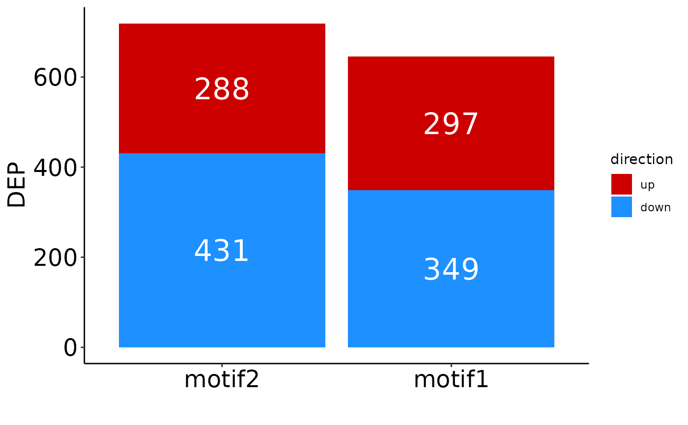
Gene set enrichment analysis (GSEA)
GSEA can be performed on the results from get_DEPresults(). This only works if the results object contains one comparison. It does not make a lot of sense to do GSEA on a DNA pull down, but this will be used for demonstration purposes nonetheless.
In addition to a results object, you need gene sets that you want to test. For this, you need to download the msigdb superset with gene sets, and extract the sets that you want. Most commonly, cancer hallmarks (h), curated gene sets (c2) and gene ontology gene sets (c5) are used. To extract these:
db <- load_msigdb(organism = 'hs') # loads the super set
#> see ?msigdb and browseVignettes('msigdb') for documentation
#> downloading 1 resources
#> retrieving 1 resource
#> loading from cache
#> require("GSEABase")
#>
#> Warning in getMsigOrganism(gsc, idType): Assuming the organism to be human.

# retrieve the cancer hallmarks
geneset_hallmarks <- get_genesets(db, collection = 'h')

# retrieve the GO:biological process gene sets.
# similarly molecular function (GOMF) and cellular compartment (GOCC) can be
# retrieved
geneset_gobp <- get_genesets(db, collection = 'c5', subcollection = 'GOBP')
To perform GSEA, use the results object and the gene sets of choice:
res <- get_DEPresults(se, 'motif1', 'neg_ctrl')
#> Tested contrasts: motif1_vs_neg_ctrl
gsea <- perform_GSEA(res, geneset_gobp)
Plotting of GSEA results
There are several options to visualize your GSEA results. The simplest is with a bar plot, showing just the Normalized Enrichment Scores (NES). The default options shows all significant results. Be specifying the top_n parameter, you can only include the n pathways with the lowest padj value.
We also remove the prefix, and shorten the names of the pathways to a maximum of 35 characters.
# Bar plot of 10 pathways with lowest padj values.
barplot <- plot_gsea_barplot(gsea, top_n = 10, remove_prefix = T,
                             max_name_length = 35)
barplot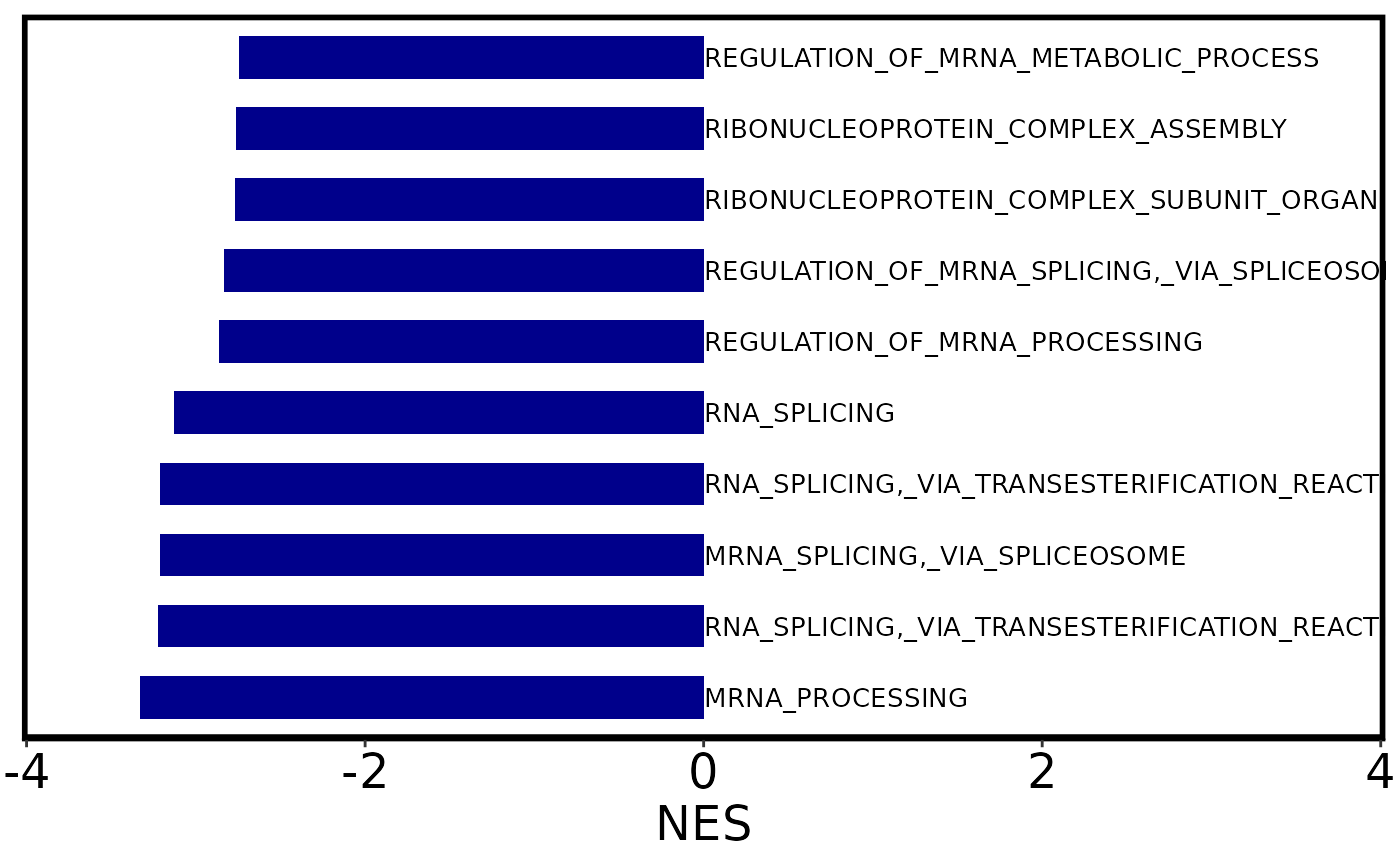
#Bar plot of 10 pathways with lowest values and different colors for bars.
barplot2 <- plot_gsea_barplot(gsea, pos_color = 'red3',
                              neg_color = 'dodgerblue', top_n = 10,
                              remove_prefix = T, max_name_length = 35)

barplot2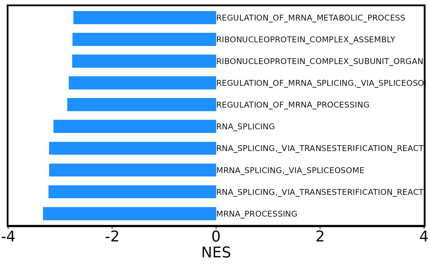
With the plot_gsea_dotplot() function, you can include more information about the pathways:
dotplot <- plot_gsea_dotplot(gsea, top_n = 10,
                             remove_prefix = T, max_name_length = 35)

dotplot
A third way way to visualize the results from GSEA is with a volcano plot with the NES on the x-axis and -log10(padj) on the y-axis. Like with the volcano plot for DEP visualization, you can specify how to label points.
# Plot all significant points (can be chaotic)
volcano <- plot_gsea_volcano(gsea)

volcano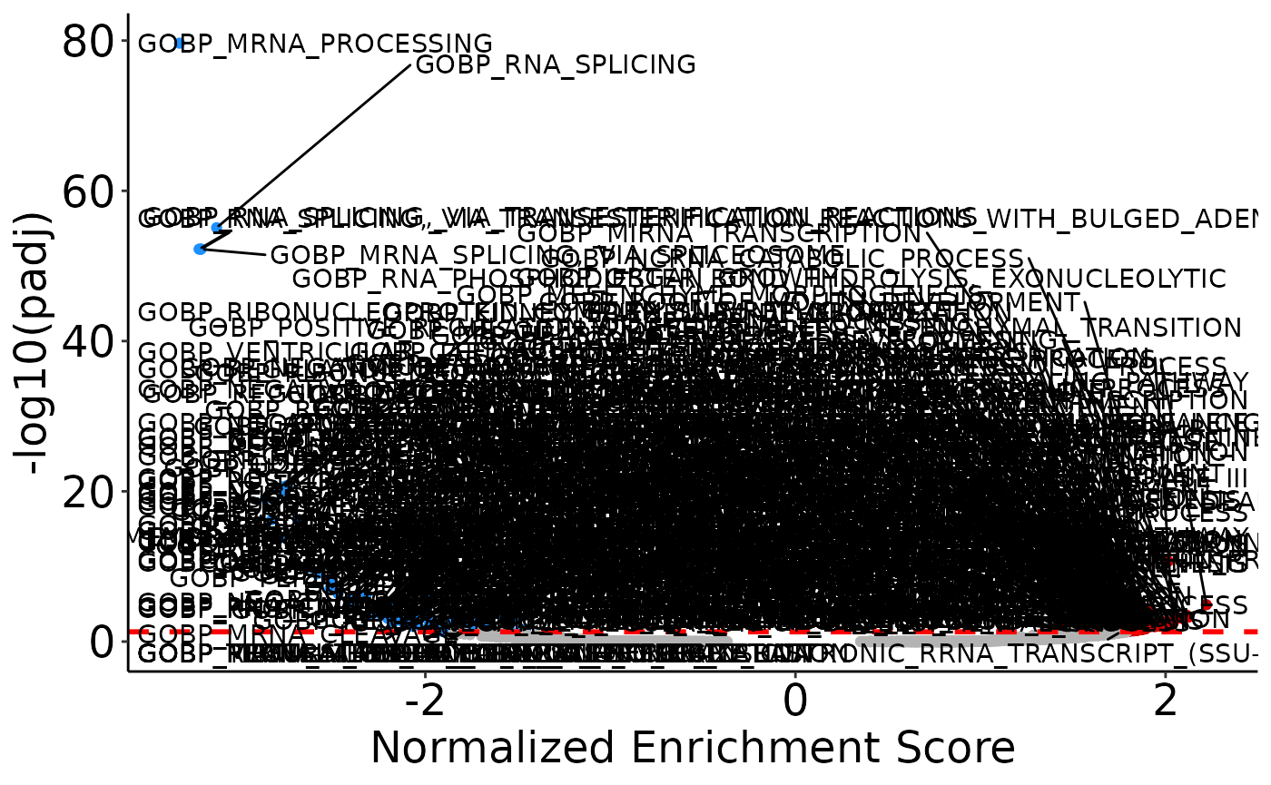
# plot 10 significant points with the lowest padj value on both sides of volcano.
volcano <- plot_gsea_volcano(gsea, top_n = 10)


volcano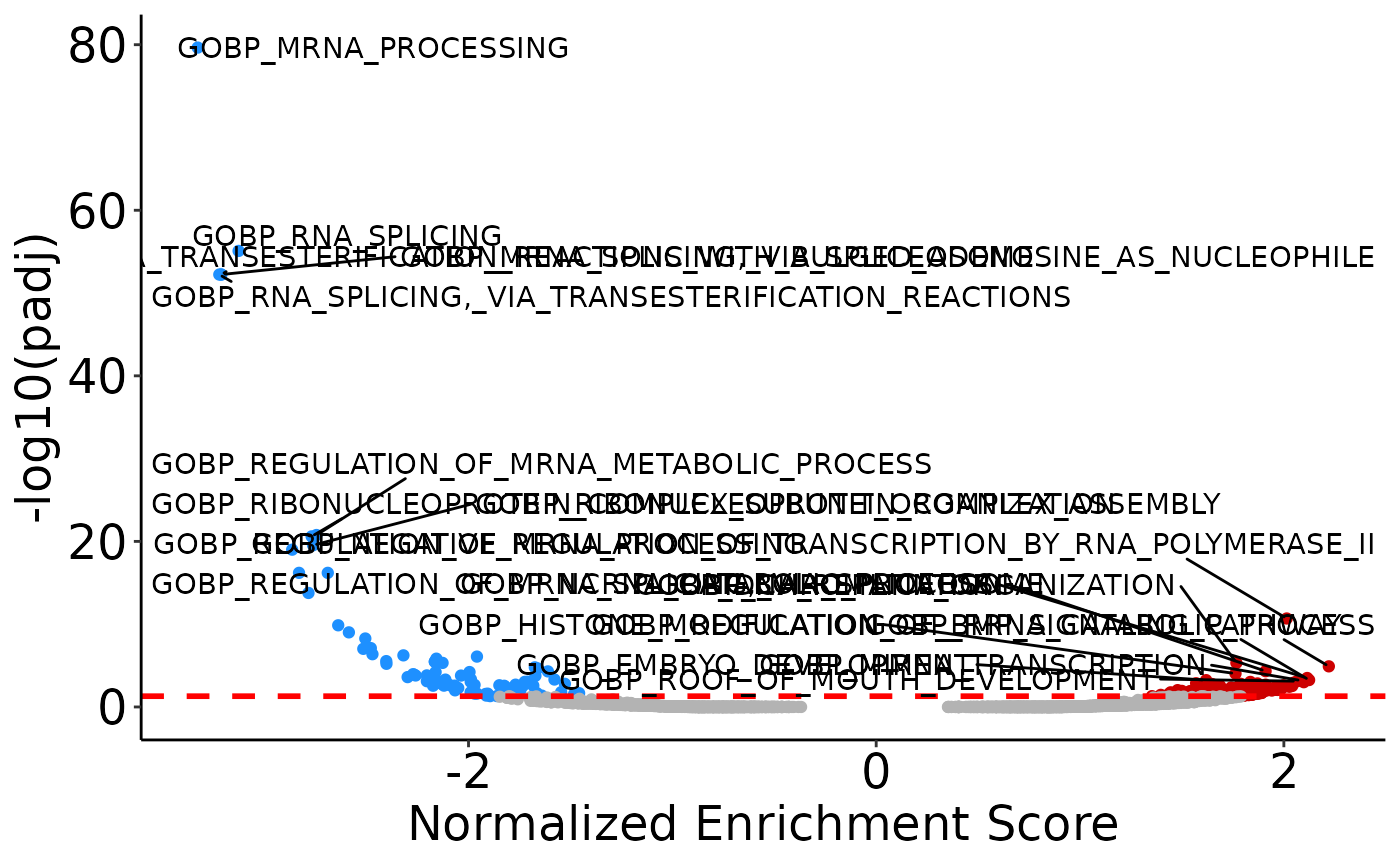
If you ran multiple GSEAs on different results objects (from get_DEPresults()), you can plot them in a single bubble plot.
res1 <- get_DEPresults(se, 'motif1', 'neg_ctrl')
#> Tested contrasts: motif1_vs_neg_ctrl
res2 <- get_DEPresults(se, 'motif2', 'neg_ctrl')
#> Tested contrasts: motif2_vs_neg_ctrl

gsea1 <- perform_GSEA(res1, geneset_gobp)
gsea2 <- perform_GSEA(res2, geneset_gobp)

bubble <- plot_gsea_bubbleplot(gsea1, gsea2,
                               sample_names = c('motif1', 'motif2'), top_n = 10,
                                remove_prefix = T, max_name_length = 35)

bubble
#> Warning: Removed 2 rows containing missing values or values outside the scale range
#> (`geom_point()`).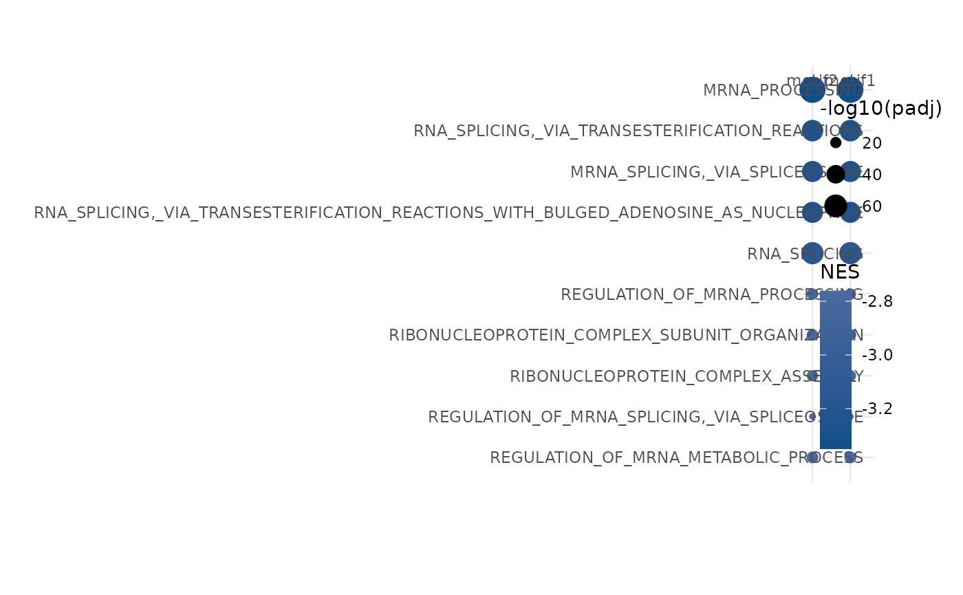
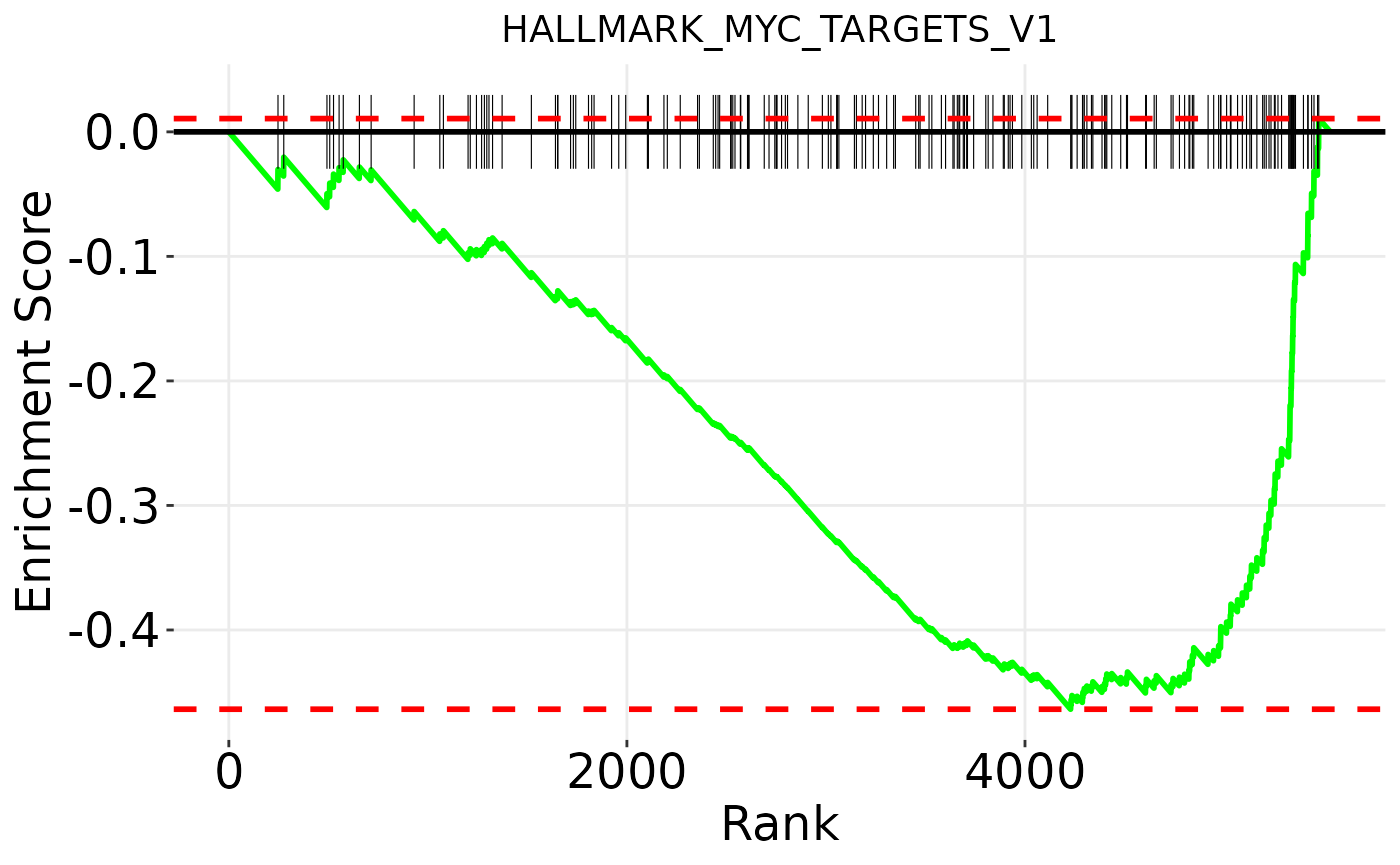
Finally, you can plot enrichment plots for individual pathways with plot_gsea_enrichment_plot():
pathways <- c('HALLMARK_MYC_TARGETS_V1', 'HALLMARK_TGF_BETA_SIGNALING')
enrichment_plots <- plot_gsea_enrichment_plot(geneset_hallmarks, pathways, res)

enrichment_plots$HALLMARK_MYC_TARGETS_V1